机器学习第一章笔记
/ / 点击 / 阅读耗时 7 分钟第一章
1.什么是模式识别
模式识别可以分为分类与回归两种
分类:输出量为离散的类别表达
回归:输出量为连续的信号表达
回归是分类的基础
2.模式识别数学表达
- 特征向量
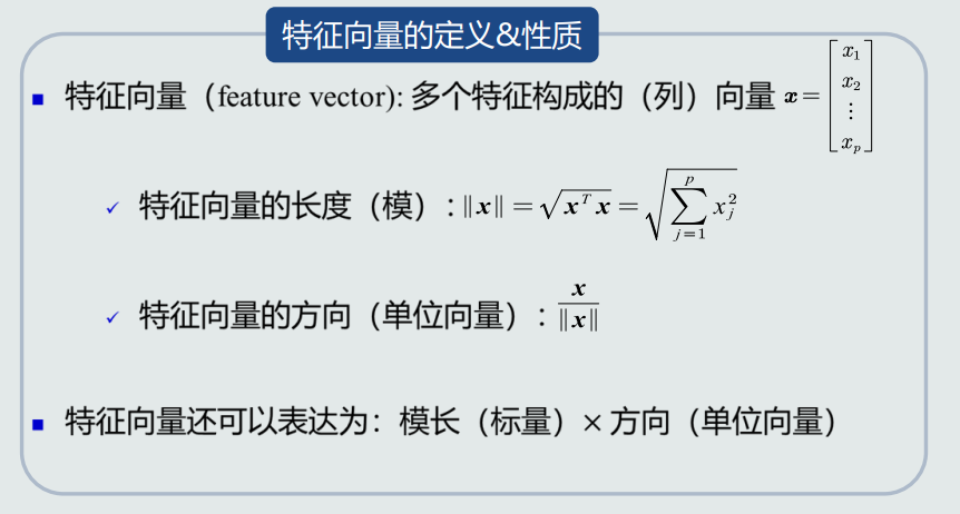
- 从坐标原点到任意一点(模式)之间的向量即为该模式的特征向量
3.特征向量的相关性
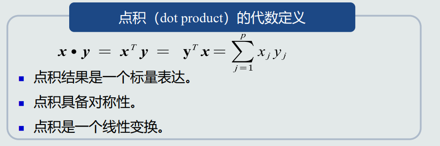
- 点积
- 投影与投影向量区别


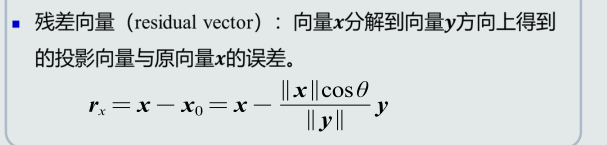
- 残差向量
4.机器学习基本概念
样本量与模型参数量
其中Over-determined:多个方程可以随意组合,解出多个解。需要loss function中加入标准,通过优化这个标准得到最优解。
Under-determined:需要在loss function中加入约束条件,得到最优解。

半监督式学习
看作有约束条件的无监督式学习问题:标注过的训练样本用作约束条件,应用在网络流数据等。
补充:
1.在从数据中提取相关特征存在困难以及标记示例对专家来说非常耗时的情况下,这种方法特别有用。
2.一种热门的训练方法是从一小组有标记数据开始训练,并使用GAN。
增强学习/强化学习
让计算机自己学习。例:马尔科夫决策(MDPs),让智能体采取行动,从而改变自己的状态获得奖励与环境发生交互的循环过程。
5.模型的泛化能力
RMSE:均方根误差
划分验证集来选择超参数
正则化
1.trade-off作用
2.提供模型唯一解的可能
6.评估方法与性能指标
留出法
1.一种方法是sklean中train_test_split
2.自己实现,用random.seed:
1
2
3
4
5
6
7
8
9
10
11
12
13
14
15
random.seed(random_seed)
data = dataset.data
target = dataset.target
# 将数据和标签绑定
all_data = np.c_[data, target]
# 随机打乱
np.random.shuffle(all_data)
print('all_data shape:', all_data.shape)
# 获取train和test集数据个数
train_size = int(all_data.shape[0] * train_ratio)
test_size = int(all_data.shape[0] * test_ratio)
# 划分train按test集
train = all_data[:train_size]
test = all_data[train_size:]K折交叉验证
1
2
3
4
5
6
7
8
9
10
11
12
13
14
15
16
17
18
19
20
21
22
23
24
25
26
27
28
29
30
31
32
num_folds = 5
k_choices = [1, 3, 5, 8, 10, 12, 15, 20, 50, 100]
X_train_folds = []
y_train_folds = []
X_train_folds = np.array_split(X_train, num_folds)
y_train_folds = np.array_split(y_train, num_folds)
k_to_accuracies = {}
classifier = KNearestNeighbor()
for k in k_choices:
k_to_accuracies[k]= []
for i in range(num_folds):
X_test_temp = np.array(X_train_folds[i])
y_test_temp = np.array(y_train_folds[i])
X_train_temp = np.array(X_train_folds[0: i] + X_train_folds[i+1: num_folds])
y_train_temp = np.array(y_train_folds[0: i] + y_train_folds[i+1: num_folds])
X_train_temp = np.reshape(X_train_temp, (X_train_temp.shape[0] * X_train_temp.shape[1], -1))
y_train_temp = np.reshape(y_train_temp, (y_train_temp.shape[0] * y_train_temp.shape[1]))
classifier.train(X_train_temp, y_train_temp)
y_test_pred = classifier.predict(X_test_temp, k=k)
num_correct = np.sum(y_test_pred == y_test_temp) / 1000
k_to_accuracies[k].append(num_correct)
for k in sorted(k_to_accuracies):
for accuracy in k_to_accuracies[k]:
print('k = %d, accuracy = %f' % (k, accuracy))准确的&精度&召回率&F1-score
1
2
3
4
5
6
7
8
9
10
11
12
13
14
15
16
17
TP, FN, FP, TN = 0, 0, 0, 0
Recall, Specificity, Precision, Accuracy, F1_score = 0., 0., 0., 0., 0.
for i in range(len(y_test)):
if y_test[i] == pos_label and y_pre[i] == pos_label:
TP += 1
elif y_test[i] == pos_label and y_pre[i] == neg_label:
FN += 1
elif y_test[i] == neg_label and y_pre[i] == pos_label:
FP += 1
elif y_test[i] == neg_label and y_pre[i] == neg_label:
TN += 1
Recall = TP / (TP + FN)
Specificity = TN / (TN + FP)
Precision = TP / (TP + FP)
Accuracy = (TP + TN) / (TP + TN + FP + FN)
F1_score = 2 * Recall * Precision / (Recall + Precision)混淆矩阵
1
2
3
4
5
6
7
8
9
10
11
12
13
14
15
16
17plt.rcParams['font.sans-serif']=['SimHei']
plt.rcParams['axes.unicode_minus'] = False
con_matrix = confusion_matrix(y_test, y_pre)
plt.figure(figsize=(14, 4), dpi=80)
plt.imshow(con_matrix, cmap=plt.cm.Blues)
indices = range(len(con_matrix))
plt.xticks(indices, [target_names[pos_label], target_names[neg_label]])
plt.yticks(indices, [target_names[pos_label], target_names[neg_label]])
plt.colorbar()
plt.xlabel('预测值')
plt.ylabel('真实值')
plt.title('混淆矩阵')
for first_index in range(len(con_matrix)):
for second_index in range(len(con_matrix[first_index])):
plt.text(first_index, second_index, con_matrix[first_index][second_index])
plt.show()PR曲线
1
2
3
4
5
6
7plt.figure("P-R Curve")
plt.title('Precision/Recall Curve')
plt.xlabel('Recall')
plt.ylabel('Precision')
precision, recall, thresholds = metrics.precision_recall_curve(y_test, y_pre)
plt.plot(recall, precision)
plt.show()ROC曲线
1
2
3
4
5
6
7
8
9
10
11
12
13
14
fpr, tpr, threshold = metrics.roc_curve(y_test, y_pre)
roc_auc = metrics.auc(fpr, tpr)
plt.figure()
lw = 2
plt.plot(fpr, tpr, color='darkorange',
lw=lw, label='ROC curve (area = %0.2f)' % roc_auc)
plt.plot([0, 1], [0, 1], color='navy', lw=lw, linestyle='--')
plt.xlim([0.0, 1.0])
plt.ylim([0.0, 1.05])
plt.xlabel('False Positive Rate')
plt.ylabel('True Positive Rate')
plt.title('Receiver operating characteristic')
plt.legend(loc="lower right")
plt.show()